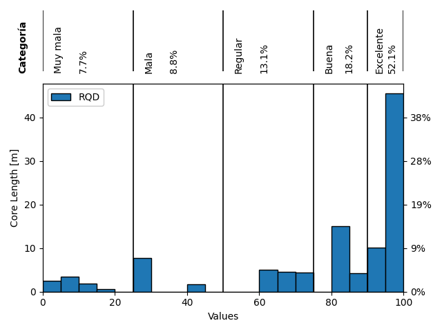
Histograms from Drill Holes Data

This example shows how to create histograms from drill holes data.

import os
import numpy as np

import geoassistant

# Path to example data
test_resources_dir = os.path.join("./resources/read_drillholes/")
collar_path = os.path.join(test_resources_dir, 'collar.csv')
survey_path = os.path.join(test_resources_dir, 'survey.csv')
geotech_log_path = os.path.join(test_resources_dir, 'drillhole_log.xlsx')

Step 1 - Load drillhole positional data

The geoassistant library provides convenient methods for reading collar and survey data. These classes allow flexible column mapping, so the CSV structure can be user-defined. The readCollarsCsvFile and readSurveysCsvFile functions return structured collections that will be used to build the full 3D drillhole geometry.

cc = geoassistant.readCollarsCsvFile(filepath=collar_path, id_key="HOLEID",
                                     x_key="X", y_key="Y", z_key="Z")

sc = geoassistant.readSurveysCsvFile(filepath=survey_path, id_key="HOLEID",
                                     dip_key="DIP", azimuth_key="AZIMUTH", depth_key="DEPTH")

Step 2 - Create drillhole geometry

Using collars and surveys, the full trajectory of each drillhole can be reconstructed. This is done through the createDrillholesFromCollarsAndSurveys method. The result is a DrillholesCollection object, which supports spatial queries, data linking, visualization, and parameter operations.

drillholes = geoassistant.createDrillholesFromCollarsAndSurveys(collars=cc, surveys=sc)

Basic info about the drillholes can now be queried directly from the object:

print(f"Number of drillholes: {len(drillholes)}")
print(f"Total length: {int(drillholes.getTotalLength()):,}")

Number of drillholes: 12
Total length: 0

See how there is no length defined? That is because geoassitant doesn’t have any reference for the length of the drillholes. This can come in various ways:

• By manually setting the length of each drill hole

• By setting the length from a log file

• By assigning the highest “To” value from a log file

Step 3 - Load geotechnical interval data

Interval-based parameters (e.g., RQD, FF) can be imported from Excel or CSV using IntervalsCollection. Each interval has a “from-to” depth and is linked to a hole ID. The column names in the spreadsheet must be specified when loading.

ic = geoassistant.readIntervalsExcelSheet(filepath=geotech_log_path, sheetname="GeotechLog",
                                          id_col='B', from_col="C", to_col="D")

Step 4 - Map parameters from the file

The raw intervals don’t contain metadata until parameter definitions are explicitly set. Here, we declare that column “L” from the Excel sheet corresponds to the “RQD” parameter.

ic.setParameterColumn(parameter_id="RQD", column="L")

Step 5 - Define computed parameters

If a parameter is derived (rather than directly mapped from a column), it can be computed manually. In this case, we define FF = n_joints / interval_length, and assign it to the interval object using setParameterValues.

n_joints = ic.getColumnValues(column="V")
lengths = ic.getLengths()
ff = np.array(n_joints) / np.array(lengths)
ic.setParameterValues(parameter_id="FF", values=ff)

Step 6 - Link intervals to drillholes

The geotechnical intervals can now be linked to the positional drillholes. This operation matches intervals to drillholes by hole ID and assigns the data accordingly. After this step, each drillhole object may contain its own set of parameters (if available).

drillholes.addIntervalsCollection(intervals=ic)

Note: Not all drillholes in the project may have matching geotechnical data. You can filter the collection to obtain only those drillholes that have a given parameter defined. Here, we get only those with FF values.

ff_drillholes = drillholes.getSubsetByParameterDefinition(parameter_id="FF")

Step 7 - Visualize the data

Using the filtered collection, we can easily generate histograms or other statistical views. In this example, we show a histogram of RQD values, but only for drillholes where FF is defined.

ff_drillholes.createParameterHistogram(parameter_id="RQD")